From Qwen-VL to Qwen3-VL: How Multimodal Models Evolved
Published:
Tags: Multimodal, Qwen, VLM
TL;DR: This article traces four generations of the Qwen-VL family. The original Qwen-VL established visual-language alignment and a three-stage training pipeline. Qwen2-VL added dynamic resolution, M-RoPE, and video input. Qwen2.5-VL focused on inference efficiency, temporal video modeling, and post-training data quality. Qwen3-VL then moved visual-language fusion deeper into the model.
Multimodal large language models (MLLMs) have become one of the busiest areas in AI research. The Qwen-VL family stands out for more than benchmark results. Its iterations follow a clear technical path, backed by practical engineering choices. From the first Qwen-VL release in 2023 to Qwen3-VL in 2025, the architecture, positional encoding, and training strategy evolved along a coherent line.
The article covers each generation in turn:
| Part | Model | Main topics |
|---|---|---|
| Part I | Qwen-VL (2023) | Three-stage training, visual-language alignment, unified multitask learning |
| Part II | Qwen2-VL (2024) | M-RoPE, 3D convolution, native dynamic resolution |
| Part III | Qwen2.5-VL (2025) | Window attention, dynamic FPS, rejection sampling and CoT |
| Part IV | Qwen3-VL (2025) | Interleaved MRoPE, DeepStack, explicit timestamps |
1. Part I: Qwen-VL, three-stage visual-language alignment (2023)
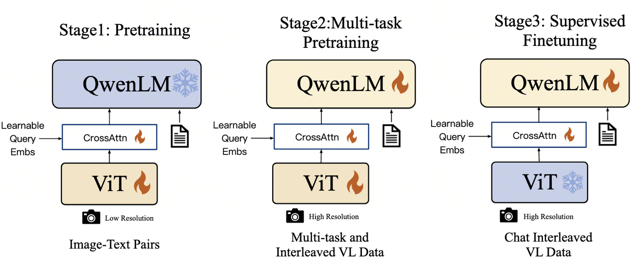
Qwen-VL started the series. Built on Qwen-7B, its main contribution was a progressive three-stage training pipeline: Align, Enhance, then Chat. Later versions changed positional encoding, video input, and training data, but kept the same broad pattern of staged training.
1.1. Training capabilities in stages
Qwen-VL gradually relaxes its training constraints. The first stage maps visual features into Qwen-7B’s language space. The second uses multitask data to add fine-grained abilities such as grounding, OCR, and VQA. The third adjusts interaction through instruction and dialogue data.
The order matters. Updating the LLM immediately with noisy web image-text pairs can damage its existing language ability. Keeping it frozen throughout training makes spatial relations, text instructions, and local visual details hard to connect. The three stages balance training stability against the depth of visual-language integration.
Their goals are:
- Align: establish a basic image-to-text mapping.
- Enhance: add grounding, OCR, chart understanding, and other capabilities through multitask learning.
- Align with Humans: turn the model into Qwen-VL-Chat, which can follow instructions and hold a dialogue.
1.2. Stage one: pre-training
The first stage has one job: train the visual encoder and adapter to compress an image into a sequence that the LLM can receive.
Most data comes from web image-text pairs in sources such as LAION, DataComp, and Coyo. The paper reports roughly 1.4 billion pairs after cleaning. The scale is large, but label quality varies. Many examples pair an image with only a short phrase, keywords, or a weak description.
The training format is simple:
<img> [visual feature sequence] </img> [text description] <eos>
The <img>...</img> markers delimit visual input. The vision encoder and adapter convert the image into 256 vectors, and the following description becomes the autoregressive target.
Qwen-7B stays frozen while the ViT and visual-language adapter are trained. This lowers cost and keeps noisy pairs from directly shifting the LLM’s language distribution. The objective remains standard text generation with cross-entropy loss: after seeing the image features, the model predicts the paired text.
This stage learns coarse alignment. It is too early to expect reliable grounding, OCR, or complex visual reasoning.
1.3. Stage two: multitask pre-training
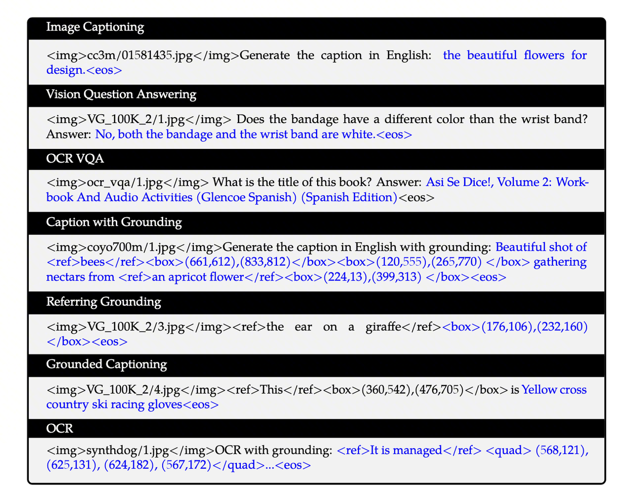
The second stage introduces high-quality human annotations across seven tasks. In the paper’s figure, black text is a prompt or context excluded from the loss, while blue text is the ground truth the model learns. Every task is cast as sequence-to-sequence text generation.
| Task | Input | Target | Training signal |
|---|---|---|---|
| Image Captioning | <img>...</img>Generate the caption in English: | the beautiful flowers for design.<eos> | Generate a description from the image |
| VQA | <img>...</img>Does the bandage have a different color than the wrist band? Answer: | No, both the bandage and the wrist band are white.<eos> | Answer a question from the image |
| OCR VQA | <img>...</img>What is the title of this book? Answer: | Asi Se Dice!, Volume 2: ...<eos> | Read visible text and answer |
| Caption with Grounding | <img>...</img>Generate the caption in English with grounding: | Beautiful shot of <ref>bees</ref><box>(...)</box> ...<eos> | Generate a caption and bounding boxes |
| Referring Grounding | <img>...</img><ref>the ear on a giraffe</ref> | <box>(176,106),(232,160)</box><eos> | Generate coordinates from a referring phrase |
| Grounded Captioning | <img>...</img><ref>This</ref><box>(360,542),(476,705)</box> is | Yellow cross country ski racing gloves<eos> | Describe the region inside a given box |
| OCR | <img>...</img>OCR with grounding: | <ref>It is managed</ref> <quad>(...)</quad>...<eos> | Recognize text and return quadrilateral coordinates |
The grounding format is the most interesting part of the table. Qwen-VL does not add a separate classification head for localization. It generates sequences such as <ref>...</ref>, <box>...</box>, and <quad>...</quad> directly. This gives up some structural priors from specialist detectors, but keeps every task within the LLM’s autoregressive training framework.
The second stage also mixes in large amounts of pure text to reduce catastrophic forgetting. The ViT, adapter, and LLM are now all unfrozen. Grounding, OCR, and chart understanding require the LLM to interpret spatial relationships and instruction intent, so visual-side updates alone are no longer enough.
The objective is still cross-entropy text generation. The difference is that targets now include answers, coordinates, OCR text, and outputs for multiple instruction formats.
1.4. Stage three: supervised fine-tuning (SFT)
The third stage produces Qwen-VL-Chat. The first two stages give the model visual and language capabilities, but do not ensure that it organizes an answer around the user’s question or follows a multi-turn dialogue format.
SFT data comes from multimodal instruction-following and dialogue datasets. Some examples are written by people, while others are produced with help from stronger models such as GPT-4. Examples use the ChatML format described in the paper and may contain one or several images across multiple turns.
The visual encoder is frozen again, leaving the adapter and LLM trainable. By this point the encoder already extracts image features. SFT mainly changes answer style, instruction following, and dialogue behavior.
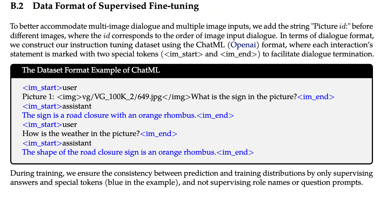
Training still uses cross-entropy text generation, but computes loss only on answers and special markers. Role names and user prompts are excluded. This makes training closer to inference, where the user’s question is context and the assistant response is what the model must predict.
Part I summary: Qwen-VL established the three-stage pipeline: connect images to Qwen-7B, add fine-grained visual skills with multitask data, and align dialogue behavior through SFT. Its limitations were equally clear. Resizing every image to 448×448 discarded detail, video had no native input path, and absolute positional encoding was poorly suited to richer multimodal coordinates. These became the main targets for Qwen2-VL.
2. Part II: Qwen2-VL, native dynamic resolution and multimodal positions (2024)
2.1. Main changes from Qwen-VL
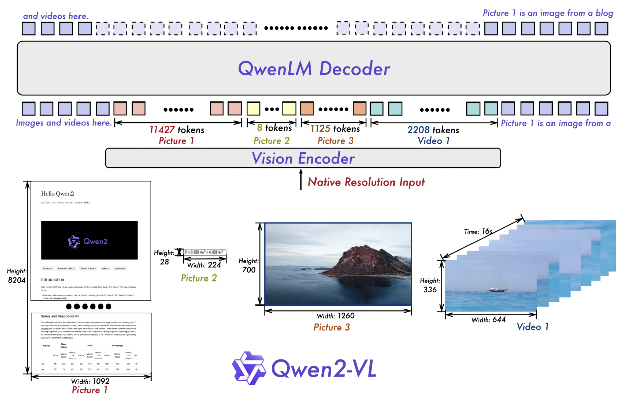
Qwen2-VL changes how inputs and positions are represented:
- It removes the original absolute position embeddings and introduces 2D-RoPE, allowing images to retain their aspect ratio and use dynamic resolution.
- It adds M-RoPE to place text, images, and video in a common spatiotemporal coordinate system.
- A depth-2 3D convolution processes video by merging 2D patches from consecutive frames into 3D tubes.
- The model supports more languages.
Qwen-VL focused on connecting an image to an LLM. Qwen2-VL focuses on consistent positional coordinates across modalities, with M-RoPE as the central design.
2.2. M-RoPE
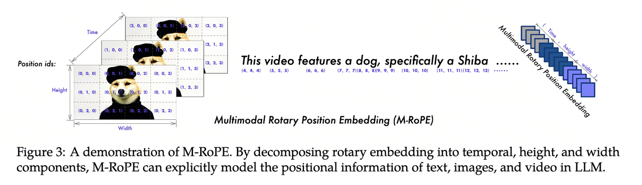
M-RoPE assigns three positional components $(t,h,w)$ to every token. Text, images, and video still enter the model as one sequence, but their positions are no longer reduced to a single index.
2.2.1. Computation
Let the input feature tensor be $X \in \mathbb{R}^{B \times L \times D}$. Every token carries a time index $P_t$, a height index $P_h$, and a width index $P_w$, each with shape $(B,L)$. For an image, time can remain constant. For text, sequence positions can be mapped onto equivalent one-dimensional coordinates.
The calculation has three steps.
- Split the hidden dimension:
- Apply RoPE to each part:
- Concatenate the original dimension:
$X_{out}$ remains $(B,L,D)$. In attention, temporal differences appear mainly in $X'_t$, while row and column differences appear in $X'_h$ and $X'_w$.
2.2.2. Problems addressed by M-RoPE
2.2.2.1. Incompatible dimensions across modalities
Text is a one-dimensional sequence, an image has two-dimensional spatial structure, and video adds time. A single flattened index mixes space and time. Separate position encodings for each modality make cross-modal fusion harder.
M-RoPE uses $(t,h,w)$ throughout:
- Text uses $(i,i,i)$ for sequential order.
- Images use $(1,h,w)$ for two-dimensional space.
- Video uses $(t,h,w)$ for space and time.
All modalities still share one embedding space for attention, while their position components retain clear meanings.
2.2.2.2. Position extrapolation in long videos
Video token counts grow quickly. A 1,000-frame video with 256 tokens per frame contains 256,000 tokens. With a one-dimensional position, $m$ exceeds 250,000.
RoPE is sensitive to positions well beyond its training length. If training covers 32k and inference reaches 250k, $\cos(m\theta)$ falls into a distribution the model has not seen.
M-RoPE splits the large index into smaller components. A sequence may contain 250,000 tokens, while $t$ reaches only 1,000 and $h$ and $w$ may reach only 16. Spatial positions remain small, and growth in time does not simultaneously disrupt spatial representation.
2.2.3. Spatiotemporal downsampling with 3D convolution
2.2.3.1. Purpose
The 3D convolution reduces the number of video tokens. Consecutive frames usually contain heavy redundancy, so processing each frame independently makes sequence length grow linearly.
Qwen2-VL merges two temporal frames into one token. Under the same token budget, the model can ideally read roughly twice as much video. For a fixed duration, the number of visual tokens is approximately halved.
2.2.3.2. Implementation
A conventional ViT can split each video frame into $14 \times 14$ patches. If one frame produces $N$ tokens, $T$ frames produce $T \times N$.
Qwen2-VL uses a 3D convolution with temporal depth 2. It processes the same spatial region in two adjacent frames at once, forming a $2 \times 14 \times 14$ tube. This also gives images and video a similar interface: an image can be duplicated into two frames, while video is compressed in two-frame groups.
2.3. Training
2.3.1. Main training setup
Qwen2-VL still uses next-token prediction. Cross-entropy loss is computed only on text tokens; visual tokens are masked with weight 0.
The LLM starts from Qwen2 at 1.5B, 7B, or 72B. The ViT starts from DFN, replaces absolute positions with 2D-RoPE, and then follows three stages.
2.3.1.1. Stage one: ViT training
The first stage trains the ViT and adapter while freezing the LLM. It uses 600B tokens, mostly large-scale weakly labeled image-text pairs. The ViT adapts to 2D-RoPE and begins aligning its visual features with Qwen2’s semantic space.
2.3.1.2. Stage two: full-parameter pre-training
The second stage unfreezes the ViT, LLM, and adapter. Another 800B tokens bring the total to 1.4T. Data includes mixed image-text examples, OCR, interleaved image-text documents, video, and pure text to preserve language ability.
Three mechanisms become active: Naive Dynamic Resolution accepts arbitrary image resolutions, M-RoPE unifies positions across text, images, and video, and 3D convolution gives images and video a common visual input form.
2.3.1.3. Stage three: instruction fine-tuning
The third stage freezes the ViT and trains the LLM. ChatML data covers multimodal conversations, long-video QA, agent action sequences, and text-only instructions. Loss also masks the <|im_start|>user portion so that only assistant responses are predicted.
Part II summary: Qwen2-VL fixes the original model’s fixed resolution and lack of native video input. M-RoPE gives text, images, and video one coordinate system; 3D convolution reduces video tokens; and dynamic resolution avoids information loss from resizing. These changes expose the next bottlenecks. High-resolution inputs make global ViT attention quadratically expensive, and video time is still represented mainly by relative frame indices rather than physical time.
3. Part III: Qwen2.5-VL, inference efficiency, time, and data quality (2025)
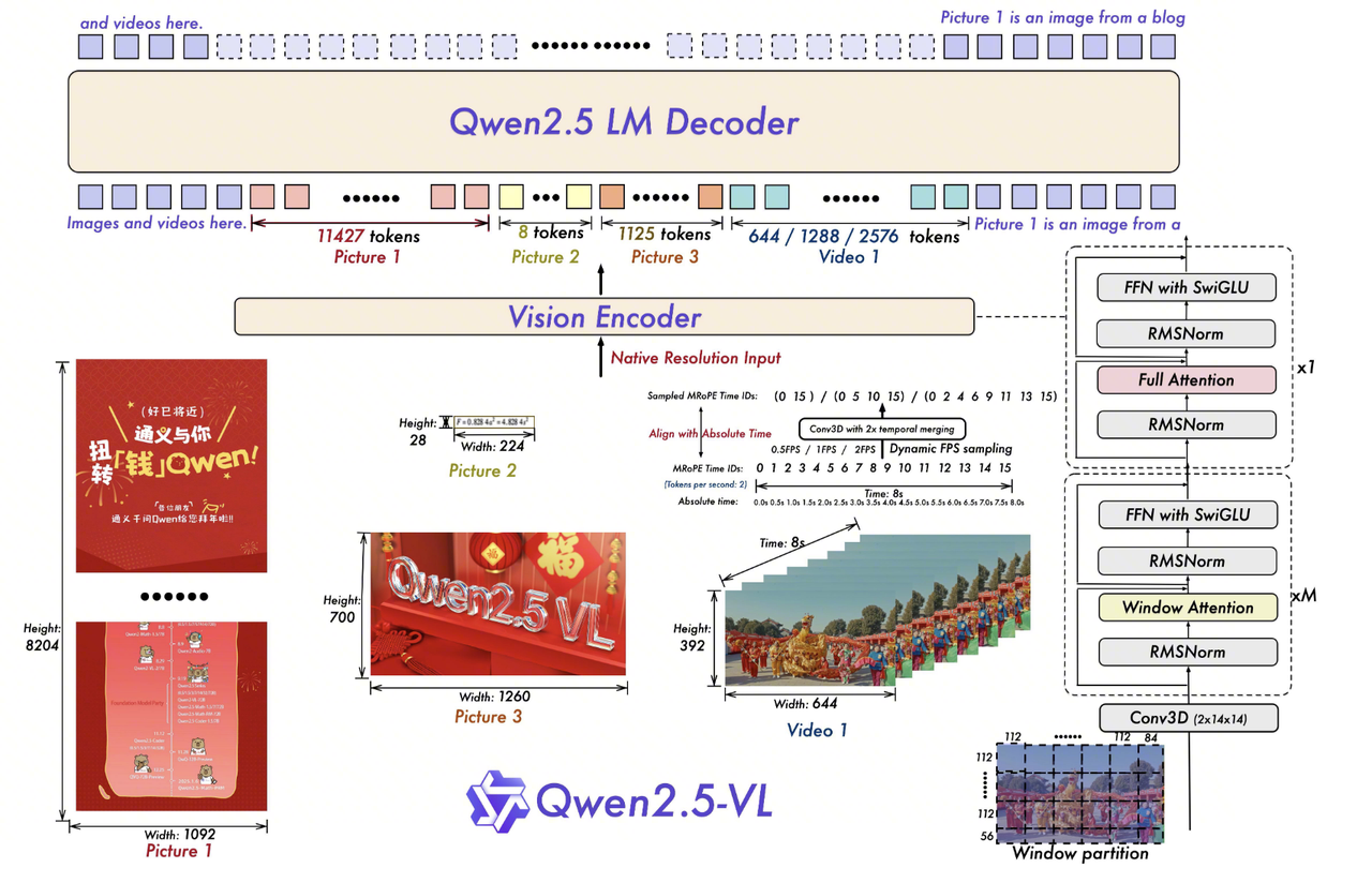
3.1. Main changes from Qwen2-VL
Qwen2.5-VL makes three groups of changes:
- Window attention reduces ViT inference cost for high-resolution images.
- Dynamic FPS extends dynamic resolution into time and supports videos sampled at different rates.
- Absolute-time MRoPE replaces relative frame numbers with position IDs tied to real time.
All three respond to one problem. Qwen2-VL can already process dynamic-resolution images and video, but high-resolution images, long videos, and irregular temporal intervals continue to increase compute and positional-encoding pressure.
3.2. Window attention
A conventional ViT applies global attention to all visual tokens at $O(N^2)$ complexity. As dynamic resolution increases, $N$ grows with image area and global attention quickly becomes the bottleneck. Qwen2.5-VL restricts most layers to local windows, making their cost closer to linear in the number of visual tokens.
3.2.1. Computation
Let an input image have size $H \times W$. Qwen2.5-VL rounds $H$ and $W$ to multiples of 28, then divides it into $14 \times 14$ patches. The token count is:
\[L = (H/14) \times (W/14)\]Flattened visual features have shape $(1,L,D)$, where $D$ is the hidden size, for example 1280.
Each window covers $112 \times 112$ pixels, or $8 \times 8 = 64$ patches. The number of windows is:
\[N_{win} = \frac{L}{8 \times 8} = \frac{L}{64}\]After partitioning, the shape can be viewed as $(N_{win},64,D)$. Self-attention runs independently inside each window:
\[\text{Attention}(Q, K, V) = \text{Softmax}\left(\frac{QK^T}{\sqrt{d_k}}\right)V\]Attention within one window has a fixed size of $64^2$, for total complexity around $N_{win} \times 64^2$. Since $N_{win}$ is proportional to $L$, the cost grows approximately linearly with image area.
Local windows weaken communication across regions. Qwen2.5-VL therefore keeps full self-attention at layers {7, 15, 23, 31}, using a few global layers to exchange information between windows.
3.3. Dynamic FPS sampling
Qwen2-VL already groups video frames into 3D tubes, but its temporal sampling needs a clearer representation. Qwen2.5-VL accepts different frame rates and lets absolute-time MRoPE record the real interval between samples.
3.3.1. Computation
Video still uses 3D tubes. Spatial patches are $14 \times 14$, and the temporal stride is 2, so every two frames are grouped. For $T$ sampled frames at resolution $H \times W$, the token count is not:
\[T \times (H/14) \times (W/14)\]but:
\[\frac{T}{2} \times (H/14) \times (W/14)\]This roughly halves the number of tokens while each token retains motion information from a short interval. The input need not use a fixed 1 FPS and may arrive at 0.5 or 2 FPS. What matters is that the position encoding records the actual time represented by each tube.
3.4. MRoPE with absolute time
Frame positions in Qwen2-VL are closer to relative frame numbers: Frame 0, Frame 1, Frame 2. They cannot distinguish whether the gap from Frame 1 to Frame 2 is 0.1 seconds or 10 seconds.
Qwen2.5-VL ties temporal position IDs to real video time. Height and width still follow MRoPE’s spatial coordinates. The temporal component represents the second in the video associated with each visual token, rather than only its frame index.
3.4.1. Computation
Every video token needs three positions:
- $ID_t$: temporal position from the frame or tube’s actual time in the video.
- $ID_h$: the row of the visual patch.
- $ID_w$: the column of the visual patch.
The calculation can be separated into four steps.
Determine timestamps after sampling. Suppose visual tube $i$ covers time $t_{abs}^{(i)}$ in seconds. This can come from sampled frame timestamps or a representative time for the pair of frames.
Map real time to a RoPE position ID. Instead of a consecutive frame number $k$, Qwen2.5-VL uses:
Here, $v$ is the number of position-ID units per second. If $v=2$, the times 0.0s, 0.5s, and 2.0s map to:
\[0,\quad 1,\quad 4\]Video position IDs may therefore jump, as in $(0,12,48)$, rather than forming the usual consecutive sequence $(0,1,2)$. Those gaps encode real temporal intervals.
- Apply MRoPE positions to separate feature subspaces. As in Qwen2-VL, split the hidden dimension into time, height, and width:
Apply the rotations:
\[X'_t = \text{RoPE}(X_t, ID_t), \quad X'_h = \text{RoPE}(X_h, ID_h), \quad X'_w = \text{RoPE}(X_w, ID_w)\]Then concatenate the feature:
\[X_{out} = \text{Concat}(X'_t, X'_h, X'_w, \text{dim}=-1)\]- Use RoPE’s relative-position property in attention. For video tokens $i$ and $j$, the temporal phase difference is set by:
Frames 0.5 seconds apart may have $\Delta_t=1$, while frames 1.5 seconds apart may have $\Delta_t=3$. The model now observes a rotation difference tied to actual elapsed time, rather than only “adjacent frames” or “two frames apart.” This distinction matters for action tempo, event order, and localization in long videos.
3.5. How the three mechanisms work together
The three mechanisms act at different points in the video pipeline.
Input compression comes first. Dynamic FPS selects frames, then each 3D tube merges the same spatial patch from two adjacent frames. For $T$ sampled frames, the count falls from $T \times H/14 \times W/14$ to $T/2 \times H/14 \times W/14$.
Temporal labeling comes next. Each tube receives $ID_t$ from its time in seconds. Two adjacent visual tokens therefore produce different temporal RoPE phases when one pair is 0.5 seconds apart and another is 2 seconds apart.
Finally, tokens with $(ID_t,ID_h,ID_w)$ enter the ViT. Most layers attend only within local $8 \times 8$ windows to extract features cheaply, while a few full-attention layers exchange information across windows.
Together, these choices handle three constraints: long video-token sequences, uneven sampling intervals, and the global-attention cost of high-resolution inputs.
3.6. Difference from Swin Transformer’s shifted windows
3.6.1. Cross-window communication
Swin Transformer communicates across windows by shifting them. Layer $l$ uses regular windows; layer $l+1$ shifts the partition so information from neighboring windows can propagate through overlap. It generally avoids explicit full-image attention.
Qwen2.5-VL does not shift its windows. Most layers use fixed, non-overlapping windows, and a few layers insert full self-attention. It replaces Swin’s alternating shifts with local windows plus occasional global layers.
3.6.2. Why not use shifted windows?
Dynamic resolution is the main reason. Shifted windows fit fixed image sizes cleanly, while Qwen2.5-VL handles varying aspect ratios and dimensions. Shifts introduce more padding and masking, and irregular boundaries make the implementation and kernels less efficient.
Fixed windows with a few global layers are more direct. The paper uses full self-attention in only four layers, keeping compute approximately linear in input size. Those layers can also use kernels such as FlashAttention to contain their practical cost.
3.7. Training
Qwen2.5-VL has five pre-training and post-training stages. Its data grows from 1.2T to 4.1T tokens, with more emphasis on high resolution, long video, reasoning data, and preference alignment.
3.7.1. Pre-training
Stage 1: visual encoder initialization
Only the redesigned ViT is trained at first; the LLM is absent or frozen. The encoder must learn a stable mapping from pixels to semantic features and begin aligning with the language space.
Data includes basic image-text pairs, visual knowledge, and OCR. Complex reasoning is not the goal yet.
Stage 2: multimodal pre-training
All parameters are unfrozen and the ViT and LLM train together. Data now includes interleaved image-text documents, VQA, multitask examples, and pure text. Text-only data continues to protect the LLM’s existing language distribution.
Context length is limited to 8,192 (8k) in this stage.
Stage 3: long-context pre-training
Full-parameter training continues as the context grows from 8k to 32,768 (32k). Long video, agent trajectories, and high-resolution documents target longer time spans, complex action sequences, and fine-grained document recognition.
Dynamic packing groups samples of different lengths in the same computation to reduce load imbalance across image sizes and improve GPU utilization.
3.7.2. Post-training
Stage 4: supervised fine-tuning
SFT freezes the ViT and fine-tunes the LLM. ChatML examples contain explicit visual embeddings. The dataset has roughly 2 million (2M) items, split evenly between text-only conversations and multimodal conversations over images and video.
Filtering matters more at this scale. Rule-based filters deduplicate and remove broken examples. Model-based filtering uses a 72B model to score samples and remove low-quality pairs whose images and text do not match.
For math, code, and some VQA tasks, Qwen2.5-VL also constructs chain-of-thought data through rejection sampling. The model produces several candidates, ground truth or a verifier removes wrong answers, and examples with both correct answers and sound reasoning return to the SFT set.
Stage 5: direct preference optimization (DPO)
DPO keeps the ViT frozen and optimizes the LLM. Each preference pair contains a better response $y_w$ and a worse response $y_l$ to the same question. The paper applies DPO to image-text and text-only data to reduce hallucination and improve preference alignment.
3.7.3. Rejection sampling
Rejection sampling is a Best-of-N data construction method. It changes where SFT examples come from rather than changing the model architecture. The model generates several candidates, then answer verification and quality filters select the examples used for training.
Qwen2.5-VL mainly uses this process for math, code generation, and domain-specific VQA:
- An intermediate Qwen2.5-VL generates $N$ responses to the same prompt.
- Each candidate receives a hard check. Math uses the final answer, code runs test cases, and VQA compares against ground truth.
- Candidates with correct answers go through another quality filter that removes code switching, repetitive patterns, excessive length, and formatting errors.
- The remaining CoT examples enter the SFT dataset.
This fills two gaps in the data. Many problem sets contain a question and final answer but no intermediate reasoning. Rejection sampling produces CoT that can be verified. Human-written reasoning can also differ from the model’s own distribution, while self-generated examples that pass verification are easier for the current model to absorb.
System prompts, format constraints, and few-shot examples can elicit the CoT. A common format is:
<thinking>
Step 1: inspect the upper-left corner of the image and find a red object...
Step 2: use its shape to identify it as an apple...
...
</thinking>
<answer>
It is an apple.
</answer>
Malformed output can be discarded or retried during sampling. A few-shot example gives the model a reasoning style to imitate:
Question: What is the area of the triangle in the image?
Answer: The base is 4 and the height is 3. Using the triangle area formula, 1/2 × base × height, the area is 1/2 × 4 × 3 = 6. The answer is 6.
Question (current task): What is the area of the circle in the image?
Answer: … (the model follows the style and steps above)
Filtering has two layers. Rules catch obviously bad samples, including meaningless switching between Chinese and English, high n-gram repetition, abnormal length, and unclosed <thinking> tags. Model-based filters cover issues that rules cannot, often using a 72B model, reward model, or verifier to score visual-text consistency, logical coherence, usefulness, and safety. Visual-text consistency is especially important for a VLM. If a CoT says there is a blue dog in the upper-left corner but the image shows a red cat, a clean reasoning format does not make it valid training data.
Part III summary: Qwen2.5-VL addresses several pressure points left by Qwen2-VL. Window attention controls the cost of high-resolution inputs. Dynamic FPS and absolute-time MRoPE improve temporal representation. The 4.1T-token corpus and rejection sampling broaden coverage and improve CoT quality. Qwen3-VL then asks where and how visual information should enter the LLM itself.
4. Part IV: Qwen3-VL, deeper visual-language fusion (2025)
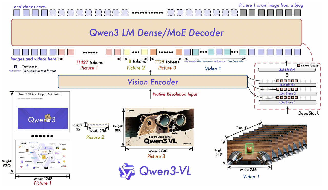
Qwen3-VL focuses on two issues exposed by Qwen2.5-VL. Blockwise MRoPE gives different axes uneven access to the frequency spectrum, while visual information enters the LLM only at its input. The main changes are Interleaved MRoPE, DeepStack, and explicit video timestamps.
4.1. Architecture changes
4.1.1. Interleaved MRoPE
Qwen2.5-VL uses standard MRoPE, assigning contiguous blocks of the position-embedding dimensions to time $t$, height $h$, and width $w$. The division is clear, but its spectrum is unbalanced: an axis may receive only a particular range of frequencies, which can limit long-video or fine-grained spatial modeling.
Interleaved MRoPE distributes components from all three axes throughout the embedding dimensions instead of placing $t$, $h$, and $w$ in separate blocks. Each spatiotemporal axis gains access to both low and high frequencies.
4.1.2. DeepStack
Conventional visual-language alignment takes the final ViT layer, projects it through an MLP, and passes the result to the LLM. The interface is simple, but visual information appears mainly at the input. Fine-grained signals such as texture and small objects may be compressed out of deep semantic features.
Inspired by Meng et al., 2024, DeepStack extracts visual tokens from several levels of SigLIP-2. After projection, features from low through high layers enter the first three LLM layers through residual connections. The model can use high-level semantics alongside lower-level visual detail without appending more visual tokens to the context, so sequence length does not increase.
4.1.3. Explicit video timestamps
Qwen2.5-VL represents absolute time through time-synchronized MRoPE, but long video creates large, sparse position IDs and ties data construction more closely to the sampling policy.
Qwen3-VL instead writes timestamps as text. It samples at a rate adapted to video length and inserts a timestamp token before each group of frames, such as <3.0 seconds>. Training mixes seconds and HMS formats:
- Seconds:
<125.5 seconds> - HMS:
<00:02:05>
Time now appears directly in the text sequence. This helps temporal localization and dense captioning while reducing dependence on a fixed frame rate.
5. Summary and outlook
5.1. How the four generations changed
The progression can be separated into the visual encoder, positional encoding, video processing, and training:
| Dimension | Qwen-VL (2023) | Qwen2-VL (2024) | Qwen2.5-VL (2025) | Qwen3-VL (2025) |
|---|---|---|---|---|
| Visual encoder | ViT + fixed resolution | ViT + native dynamic resolution | ViT + window attention | SigLIP-2 + DeepStack |
| Position encoding | Absolute positions | Blockwise M-RoPE | M-RoPE + absolute time | Interleaved MRoPE |
| Video | Unsupported | 3D convolution for spatiotemporal downsampling | Dynamic FPS | Explicit text timestamps |
| Training | Three-stage progressive training | Three stages: ViT → full parameters → SFT | Five stages, adding long context and DPO | Continues and deepens the pipeline |
| Main change | Establishes the training pipeline | Unifies multimodal positions | Improves inference efficiency and data quality | Adds deeper visual fusion |
5.2. Recurring design choices
Several ideas continue across all four generations:
Training stability comes first: later components are unfrozen only after the visual side has begun to align, and complex joint training follows.
One serialized interface: grounding coordinates, OCR text, and video timestamps are represented as text whenever possible, reusing the LLM’s autoregressive machinery.
Time becomes more explicit: video progresses from no native support, to relative frame indices, to absolute-time position encoding, and finally to text timestamps.
Data quality gains weight: web image-text pairs give way to multitask annotations and then verified CoT from rejection sampling. Data engineering becomes increasingly important in later generations.
5.3. What remains open
DeepStack shifts the question from where to attach a visual encoder to which visual granularity should enter which LLM layers. Explicit timestamps also show that a longer context window alone does not solve video understanding. The time representation and sampling policy affect localization and long-video captioning directly.
Two questions stand out to me. The first is whether deep visual injection introduces training instability or interference between modalities. The second is how explicit timestamps generalize across sampling rates and long-video QA tasks.
6. Further reading
The following papers cover the techniques discussed above.
Visual encoders
An Image is Worth 16x16 Words: Transformers for Image Recognition at Scale (ViT, Dosovitskiy et al., 2020), the visual backbone behind the Qwen-VL family and the basic formulation of images as Transformer patch sequences.
Swin Transformer: Hierarchical Vision Transformer using Shifted Windows (Liu et al., 2021), the main comparison for Qwen2.5-VL’s window attention. Swin’s shifted windows provide a useful contrast with fixed 2D-RoPE windows plus occasional global layers.
Sigmoid Loss for Language Image Pre-Training (SigLIP, Zhai et al., 2023), background for Qwen3-VL’s move to SigLIP-2. SigLIP replaces the softmax contrastive objective with a sigmoid loss.
Positional encoding and sequence modeling
RoFormer: Enhanced Transformer with Rotary Position Embedding (Su et al., 2021), the theoretical basis for M-RoPE. Several Qwen-VL generations depend on RoPE’s relative-position property.
ViViT: A Video Vision Transformer (Arnab et al., 2021), useful background for Qwen2-VL’s temporal downsampling through 3D convolution and for the wider design space of video ViTs.
Visual-language fusion
Flamingo: a Visual Language Model for Few-Shot Learning (Alayrac et al., 2022), an important multimodal model whose cross-attention design provides context for DeepStack’s deeper fusion.
DeepStack: Deeply Stacking Visual Tokens is Surprisingly Simple and Effective for LMMs (Meng et al., 2024), a direct reference for Qwen3-VL that injects groups of visual tokens at different LLM layers.
Visual Instruction Tuning (LLaVA, Liu et al., 2023), a representative visual instruction-tuning paper that established the now-common visual encoder, projection layer, and LLM architecture.
Training and alignment
Direct Preference Optimization: Your Language Model is Secretly a Reward Model (DPO, Rafailov et al., 2023), a training method used by Qwen2.5-VL that optimizes a policy directly from preference data without an explicit reward model.
Self-Rewarding Language Models (Yuan et al., 2024), related to Qwen2.5-VL’s rejection sampling through model self-evaluation and iterative improvement.
Dynamic resolution
- Patch n’ Pack: NaViT, a Vision Transformer for any Aspect Ratio and Resolution (Dehghani et al., 2023), background for Qwen2-VL’s native dynamic resolution. NaViT uses sequence packing to support arbitrary input sizes.
Contemporary alternatives
- InternVL: Scaling up Vision Foundation Models and Aligning for Generic Visual-Linguistic Tasks (Chen et al., 2023), a representative model with a 6B-parameter visual encoder and a useful architectural and training comparison with Qwen-VL.
Recommended: Jianlin Su’s blog Scientific Spaces has detailed articles on RoPE derivations, NTK-aware extrapolation, and multimodal positional encoding. They are particularly useful for understanding M-RoPE and its variants.
These are my personal notes on the papers. Corrections are welcome.
Leave a Comment